Analysing bibliographical references with R
Plots and wordclouds on the references gathered during my PhD thesis
During my PhD, I worked at the intersection between biophysics and plant development. My PhD topic was focused on the study of the contribution of mechanical stress to cell division. To explore this topic, I did a lot of confocal microscopy, but also a lot of bioimage analysis and data analysis. I was curious to see how the bibliography I gathered during this period reflects my PhD topic. To analyse these data, I used the R software.
Part of my work as a researcher consists in reading research articles to broaden my knowledge and keep up to date with ongoing research progresses in my field. I use Zotero to store all the references to the articles I have in my bibliography repository. During my PhD, I was using an extension from Zotero, Paper Machines, to create wordclouds. I enjoyed visualising the most frequent words present in my bibliography. Unfortunately, Paper Machines is no longer maintained. This lead me to search how to create wordclouds with R, but also at how to explore bibliography data in general. In this article, I gather my findings and propose a few examples of graphical visualisation of the bibliography ressources I gathered during my PhD. I was inspired by two other blog articles: https://davidtingle.com/misc/bib and https://www.littlemissdata.com/blog/wordclouds, and by the {bib2f} vignette https://cran.r-project.org/web/packages/bib2df/vignettes/bib2df.html
Packages
To explore the bibliography entries, I use the packages {bib2df}, {dplyr}, {tidyr}, {ggplot2} and {ggthemes}. {bib2df} allows to convert directly bib entries into a dataframe, which simplifies a lot data manipulation afterwards. I use {dplyr} and {tidyr} to do data wrangling and {ggplot2} for the data visualisation.
To construct the wordclouds from the titles of my bibliography entries, I use the packages {tm}, {wordcloud} and {wordcloud2}. {tm} allows to apply transformation functions to a text document. It is useful to remove accents, punctuation marks, capital letters… {wordcloud} and {wordcloud2} construct wordclouds from text documents. {wordcloud2} can use a binary image as a mask to shape the wordcloud. All packages can be installed from CRAN, except {wordcloud2}, which requires the development version on GitHub.
library(bib2df)
library(dplyr)
library(tidyr)
library(ggplot2)

library(tm)
library(wordcloud)
# devtools::install_github("lchiffon/wordcloud2")
library(wordcloud2)

library(glue)
library(forcats)
Plots: Theme and palette
The code below defines a common theme and color palette for all the plots.
# Define a personnal theme
custom_plot_theme <- function(...){
theme_bw() +
theme(panel.grid = element_blank(),
      axis.line = element_line(size = .7, color = "black"),
axis.text = element_text(size = 11),
axis.title = element_text(size = 12),
legend.text = element_text(size = 11),
legend.title = element_text(size = 12),
legend.key.size = unit(0.4, "cm"),
strip.text.x = element_text(size = 12, colour = "black", angle = 0),
strip.text.y = element_text(size = 12, colour = "black", angle = 90))
}

# Define a palette for graphs
greenpal <- colorRampPalette(brewer.pal(9,"Greens"))
Loading the bibliography data
First, let’s use the {bib2df} package to load the .bib file containing all the bibliography references I gathered during my PhD. This file contains more references than what I actually cited in my PhD manuscript. The .bib file can be downloaded here.
myBib <- "PhD_Thesis.bib"df_orig <- bib2df(myBib)
head(df_orig)## # A tibble: 6 x 35
## CATEGORY BIBTEXKEY ADDRESS ANNOTE AUTHOR BOOKTITLE CHAPTER CROSSREF
## <chr> <chr> <chr> <chr> <list> <chr> <chr> <chr>
## 1 ARTICLE enugutti_reg… <NA> <NA> <chr [… <NA> <NA> <NA>
## 2 ARTICLE dumais_analy… <NA> <NA> <chr [… <NA> <NA> <NA>
## 3 ARTICLE sawidis_pres… <NA> <NA> <chr [… <NA> <NA> <NA>
## 4 ARTICLE chen_geometr… <NA> <NA> <chr [… <NA> <NA> <NA>
## 5 ARTICLE harrison_com… <NA> <NA> <chr [… <NA> <NA> <NA>
## 6 ARTICLE uyttewaal_me… <NA> <NA> <chr [… <NA> <NA> <NA>
## # ... with 27 more variables: EDITION <chr>, EDITOR <list>,
## # HOWPUBLISHED <chr>, INSTITUTION <chr>, JOURNAL <chr>, KEY <chr>,
## # MONTH <chr>, NOTE <chr>, NUMBER <chr>, ORGANIZATION <chr>,
## # PAGES <chr>, PUBLISHER <chr>, SCHOOL <chr>, SERIES <chr>, TITLE <chr>,
## # TYPE <chr>, VOLUME <chr>, YEAR <dbl>, URL <chr>, URLDATE <chr>,
## # KEYWORDS <chr>, FILE <chr>, SHORTTITLE <chr>, DOI <chr>, ISSN <chr>,
## # ISBN <chr>, LANGUAGE <chr>Tidying the bibliography entries
A closer look to the JOURNAL column reveals that the naming of the journals is not consistent. As this will bias future analyses of the data, it is important to spot the journals for which the name exists in different formats and to correct them.
journal_names <- unique(df_orig$JOURNAL)
head(journal_names)
## [1] "Proceedings of the National Academy of Sciences"
## [2] "The Plant Journal"
## [3] "Protoplasma"
## [4] "Science"
## [5] "Faraday Discussions"
## [6] "Cell"I found a few journal names written in several ways. For instance: “PNAS”, “Proceedings of the National Academy of Sciences” and “Proceedings of the National Academy of Sciences of the United States of America” correspond to the same journal. To clean the data, I looked at the names of the journals one by one and tried to spot as much synonyms as possible. To reduce the number of synonyms, I started by lowering letter case, removing extra spaces and some special characters. Note that, ideally, this data curation should be done in the raw dataset in Zotero to keep an homogeneous bibliography…
df <- df_orig %>%
  # clean names
  mutate(JOURNAL = tolower(JOURNAL) %>%
           gsub("\\s+", " ", .) %>%
           gsub("\\\\", "", .) %>%
           gsub("\\&", "and", .)) %>%
  # replace synonyms
  mutate(JOURNAL = case_when(
    JOURNAL == "nature rewiews molecular cell biology" ~ "nature reviews molecular cell biology",
    grepl("proceedings of the national academy of sciences", JOURNAL) ~ "pnas",
    grepl("proceedings of the national academy of sciences of the united states of america", JOURNAL) ~ "pnas",
    grepl("the plant cell online", JOURNAL) ~ "the plant cell",
    TRUE ~ JOURNAL
    ))
To check the tidyness of the data, I could also look at the names of the authors, the years, which are sometimes missing or weird, and the “BIBTEXKEY” column, which should contain unique bibliography entries, unless there is duplicates. Moreover, for the overall tidyness of the Zotero database, it can also be useful to find the entries having only a few or no keywords. Keywords are very useful to find back bibliographical entries quickly in Zotero, but it is easy to forget to populate them.
Exploring the bibliography data
Category
Let’s first have a look at all the category of the publications that are in my bibliography. I am expecting a high number of research articles, but I know I also have a few R packages for instance.
count(df, CATEGORY, sort = TRUE)| CATEGORY | n |
|---|---|
| ARTICLE | 453 |
| MISC | 9 |
| INCOLLECTION | 4 |
| BOOK | 2 |
| INPROCEEDINGS | 2 |
| PHDTHESIS | 1 |
Without surprise, most of the publications in my PhD bibliography collection are research articles. There is also two books. In my bibliography, the publications in “INCOLLECTION” correspond to book sections and the one in “INPROCEEDINGS” to conference papers. To finish, the “MISC” category corresponds to the R, Matlab and GIMP softwares, and to the major R packages I used. The Fiji image analysis software is cited as a research article.
This data mining is an opportunity for me to remind you that it is important to mention the softwares, but also the packages and plugins used in scientific articles, especially those that are free and open-source. Citations are currently often the only way to ensure continuity of funding for these tools.
filter(df, CATEGORY == "MISC") %>%
  mutate(TITLE = gsub("\\{|\\}", "", TITLE)) %>%
  select(TITLE)
## # A tibble: 9 x 1
## TITLE
## <chr>
## 1 R: A Language and Environment for Statistical Computing
## 2 Matlab
## 3 GNU Image Manipulation Program
## 4 moments: Moments, cumulants, skewness, kurtosis and related tests
## 5 raster: Geographic Data Analysis and Modeling
## 6 FactoMineR: Multivariate Exploratory Data Analysis and Data Mining
## 7 RImageJROI: Read 'ImageJ' Region of Interest (ROI) Files
## 8 snow: Simple Network of Workstations
## 9 rgl: 3D visualization device system (OpenGL)Journal
I am curious to find what is the most common journal in my PhD bibliography. I am doing this exploration for fun, but I could use this information to know better where I am usually finding my bibliography ressources, maybe reinforce this bias by suscribing to newsletters or RSS feeds from these journals (as they are my major source of information) or on the contrary, choose to diversify more my sources. I’ll filter the data to keep only the ones having a journal name, count how many occurences of the journal name there are, and arrange in descending order to see the most common journals first. Let’s see what is the top ten.
top_ten_journals <- df %>%
  filter(!is.na(JOURNAL)) %>%
  group_by(JOURNAL) %>%
  summarize(n = n()) %>%
  arrange(desc(n)) %>%
  top_n(10, n)

ggplot(top_ten_journals) +
  geom_col(aes(fct_reorder(JOURNAL, n), n, fill = n),
           colour = "grey30", width = 1) +
  labs(x = "", y = "", title = "Top 10 journals in my bibliography") +
  coord_flip() +
  scale_fill_gradientn("n", colours = greenpal(10)) +
  scale_y_continuous(expand = c(0, 0)) +
  scale_x_discrete(expand = c(0, 0)) +
  custom_plot_theme()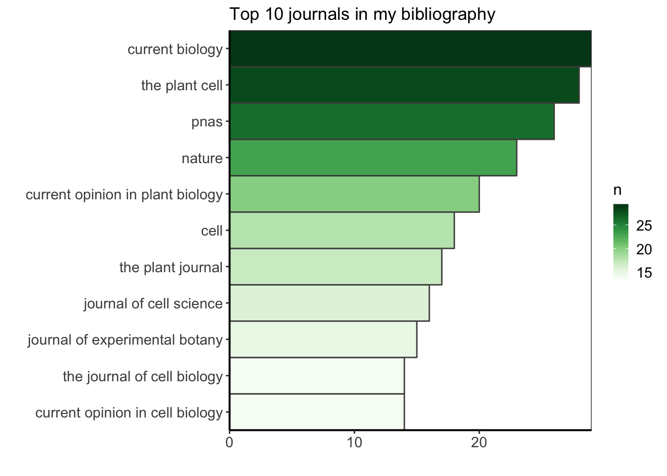
Year
Another interesting metric is the median year of the publications in my PhD bibliography. Did I mostly gathered recent papers? I will compare this median year to the year at which I submitted my PhD thesis and defended (2015) and calculate the median time between 2015 and the year of publication of the paper.
year_pub <- df %>%
  filter(is.na(YEAR) == FALSE) %>%
  mutate(YEAR = as.numeric(YEAR)) %>%
  mutate(age = 2015 - YEAR) %>%
  summarize(median_age = median(age),
            median_year = median(YEAR))
year_pub
## # A tibble: 1 x 2
## median_age median_year
## <dbl> <dbl>
## 1 6 2009Half of the publications were 6 years old or less at the time of submission of my PhD manuscript, which means that I mainly gathered recent publications in my bibliography.
Let’s now plot the number of publication per year to see how is the distribution, and let’s position the median year of publications with a vertical line.
df %>%
  filter(is.na(YEAR) == FALSE) %>%
ggplot(aes(x = as.numeric(YEAR))) +
  geom_bar(width = 1, fill = greenpal(6)[4]) +
  geom_vline(data = year_pub, aes(xintercept = median_year),
             colour = "grey30", size = 2) +
  labs(x = "", y = "") +
  ggtitle("Number of publication per year") +
  custom_plot_theme() +
  theme(axis.text.x = element_text(angle = 45, hjust = 1))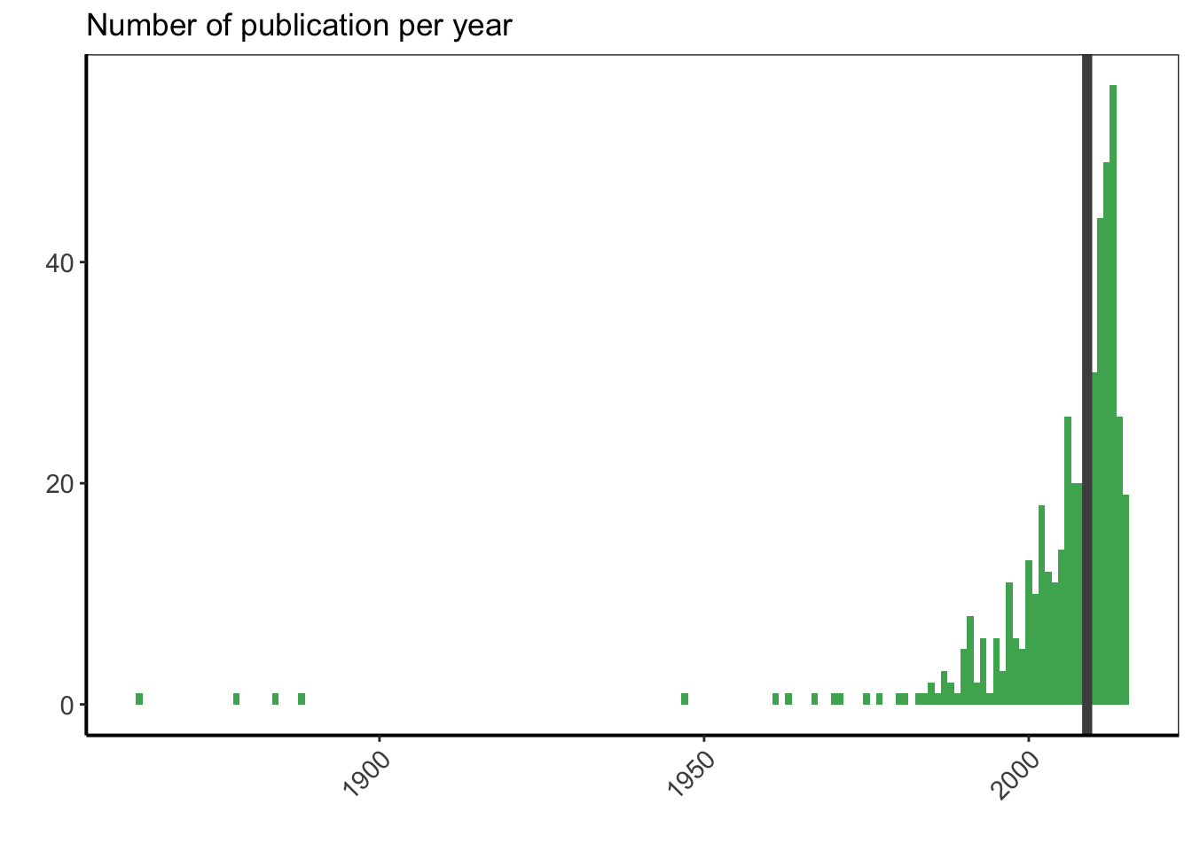
The oldest publications correspond to the cell division rules from the XIXth century. Then, I have one article from 1947, and all the rest of the publications I have are from after 1950. Half of them were even published in 2009 or after. It is not surprising to see more recent publications, as the number of publications per year continuously increased between the 50s and now, and as the most recent publications are more easily accessible online. However, I am surprised to see that the median year is only 6 years before my PhD manuscript submission.
Authors
I am curious to see who are the most frequent authors in my publication list. The initials of the first name are prone to typos as they were often entered manually. Some might be missing (in the case of multiple names, for instance). We will start using only the family name.
top_ten <- df %>%
  select(AUTHOR) %>%
  unnest() %>%
  extract(AUTHOR, into = "familyName", regex = "(.*)(?=,)") %>%
  mutate(familyName = tolower(familyName)) %>%
  count(familyName) %>%
  arrange(desc(n)) %>%
  top_n(10, n)

top_ten
## # A tibble: 10 x 2
## familyName n
## <chr> <int>
## 1 traas 25
## 2 hamant 23
## 3 lloyd 18
## 4 meyerowitz 16
## 5 boudaoud 15
## 6 smith 15
## 7 wasteneys 12
## 8 wang 10
## 9 gibson 9
## 10 li 9The risk of using only the family name is that common family names such as Smith, Li, Gibson or Wang are all attributed to the same person. To avoid this issue, I can add the initials, keeping in mind that they might be more prone to typos than the family name itself. To limit that risk, I’ll remove all punctuation signs and only keep the first initial.
top_ten_with_initials <- df %>%
  select(AUTHOR) %>%
  unnest() %>%
  extract(AUTHOR, into = c("familyName", "initials"), regex = "(.*)(?=,)(.*)") %>%
  mutate(familyName = tolower(familyName)) %>%
  mutate(initials = toupper(initials) %>%
           gsub(pattern = "[[:punct:]]", replacement = " ") %>%
           gsub(initials, pattern = " ", replacement = "") %>%
           substr(1,1)) %>%
  group_by(familyName, initials) %>%
  count(familyName) %>%
  ungroup() %>%
  mutate(name =
           glue("{substr(toupper(familyName), 1, 1)}",
                "{substr(familyName, 2, nchar(familyName))}, {initials}.")) %>%
  arrange(desc(n)) %>%
  top_n(10, n)

ggplot(top_ten_with_initials) +
  geom_col(aes(fct_reorder(name, n), n, fill = n),
           colour = "grey30", width = 1) +
  labs(x = "", y = "", title = "Top 10 authors in my bibliography") +
  coord_flip() +
  scale_fill_gradientn("n", colours = greenpal(10)) +
  scale_y_continuous(expand = c(0, 0)) +
  scale_x_discrete(expand = c(0, 0)) +
  custom_plot_theme()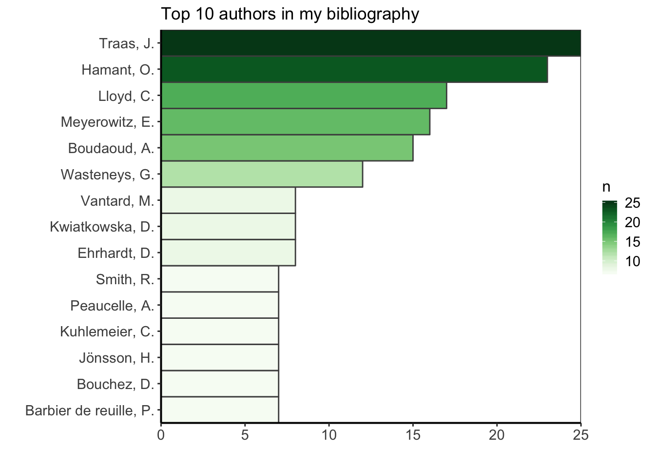
If we add the first initial, we see that “Smith” remains in the top ten but has now only 7 citations (the other 8 belonging to other “Smith” with other initials), while “Li” is not part of the top ten anymore. In the same way as for the journal names, in order to have good quality data, it would be necessary to check the authors names one by one.
Wordcloud: quick start
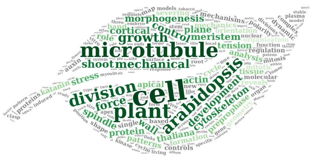
To visualise the main topic of my PhD bibliography, a wordcloud is one of the most appropriate data visualisation, as the size of the words in the cloud directly reflects their importance. Here I will use only the title of the publications for my corpus.
For a quick start, I will only use the {tm} and {wordcloud} librairies.
pubcorpus <- Corpus(VectorSource(df$TITLE)) %>%
 tm_map(content_transformer(tolower)) %>%
 tm_map(removePunctuation) %>%
 tm_map(removeWords, stopwords('english'))
my_wordcloud1 <- wordcloud(pubcorpus, max.words = 200, random.order = FALSE)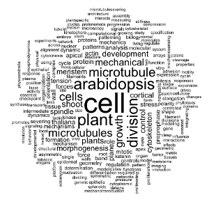
Wordcloud: advanced version
Above, I tidied quickly the corpus by setting all letters to lower case and removing the punctuation marks. In this second part, I’ll do a more in-depth cleaning of the corpus before creating the wordcloud. Again, my corpus is based on the titles of the publications in my PhD bibliography. I’ll reuse the package {wordcloud} and use also the package {wordcloud2}. {wordcloud2} allows to use a binary mask to shape the wordcloud.
docs <- SimpleCorpus(VectorSource(df$TITLE),
                     control = list(language = "en"))
If we inspect the corpus, we immediately see that it needs to be cleaned a bit: there is punctuation marks, upper and lower cases, linking words…
inspect(docs)Text transformation
To modify a text document, for instance to replace special characters, we can use the function tm_map from the package {tm}. tm_map applies a given transformation to a corpus and give back the modified corpus. To create our own transformations, we can use the function content_transformer from the package {tm}. The syntax is the following (in upper case the part to modify):
CHOOSE MEANINGFUL NAME <- content_transformer(
  function(x , pattern ) gsub(pattern, CHOOSE REPLACEMENT, x))
)
Removing punctuation
toSpace <- content_transformer(
  function(x , pattern ) gsub(pattern, " ", x))
docs <- tm_map(docs, toSpace, "[[:punct:]]")
Removing accents
toNoAccent <- content_transformer(
  function(x , pattern ) gsub(pattern, "a", x))
docs <- tm_map(docs, toNoAccent, "à|ä|â")
toNoAccent <- content_transformer(
  function(x , pattern ) gsub(pattern, "e", x))
docs <- tm_map(docs, toNoAccent, "è|é|ê|ë")
toNoAccent <- content_transformer(
  function(x , pattern ) gsub(pattern, "o", x))
docs <- tm_map(docs, toNoAccent, "ô|ö")
toNoAccent <- content_transformer(
  function(x , pattern ) gsub(pattern, "u", x))
docs <- tm_map(docs, toNoAccent, "û|ü")
toNoAccent <- content_transformer(
  function(x , pattern ) gsub(pattern, "i", x))
docs <- tm_map(docs, toNoAccent, "î|ï")
toNoAccent <- content_transformer(
  function(x , pattern ) gsub(pattern, "oe", x))
docs <- tm_map(docs, toNoAccent, "œ")
Converting the text to lower case
docs <- tm_map(docs, content_transformer(tolower))Removing alone numbers
docs <- tm_map(docs, toSpace, " [[:digit:]]* ")Removing english common stopwords
docs <- tm_map(docs, removeWords, stopwords("english"))Removing my own stop word
rm_words <- c("using")
docs <- tm_map(docs, removeWords, rm_words)
For a non scientific corpus we could use the package {pluralize}, but here it does not work well with the scientific words such as microtubules/microtubule.
tosingular <- content_transformer(
  function(x, pattern, replacement) gsub(pattern, replacement, x)
  )

docs <- tm_map(docs, tosingular, "plants", "plant")
docs <- tm_map(docs, tosingular, "microtubules", "microtubule")
docs <- tm_map(docs, tosingular, "cells", "cell")
docs <- tm_map(docs, tosingular, "forces", "force")
docs <- tm_map(docs, tosingular, "walls", "wall")
docs <- tm_map(docs, tosingular, "divisions", "division")
docs <- tm_map(docs, tosingular, "models", "model")
docs <- tm_map(docs, tosingular, "proteins", "protein")
docs <- tm_map(docs, tosingular, "dynamics", "dynamic")
Eliminating extra white spaces
docs <- tm_map(docs, stripWhitespace)Term-document matrix
The term-document matrix is a contigency table with all the words and their counts. Now that the corpus is clean, we can have a look at the top ten words used in the publication titles.
dtm <- TermDocumentMatrix(docs)
m <- as.matrix(dtm)
v <- sort(rowSums(m), decreasing = TRUE)
d <- data.frame(word = names(v), freq = v)

d %>%
  top_n(10, freq) %>%
ggplot() +
  geom_col(aes(fct_reorder(word, freq), freq, fill = freq),
           colour = "grey30", width = 1) +
  labs(x = "", y = "", title = "Top 10 words") +
  coord_flip() +
  scale_fill_gradientn("freq", colours = greenpal(10)) +
  scale_y_continuous(expand = c(0, 0)) +
  scale_x_discrete(expand = c(0, 0)) +
  custom_plot_theme()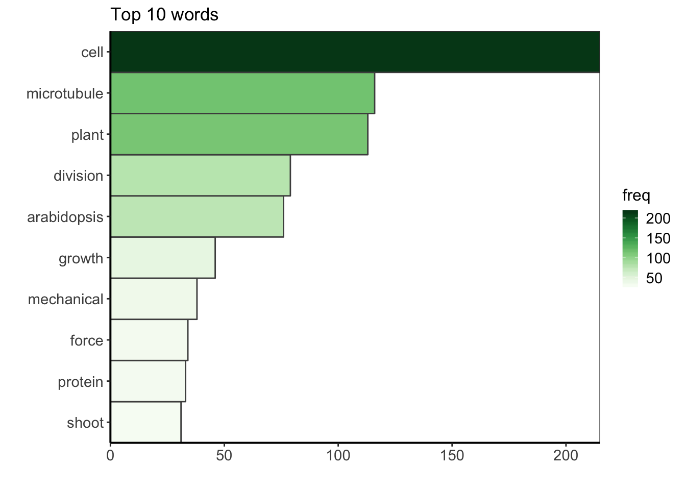
The most common word in in the corpus is the word “cell”. During my PhD I worked on cell division in plants, i.e. how one plant cell partition its volume to make two daughter cells. More precisely, I tried to understand to which extent the mechanical stress within the growing plant tissue can affect this partitionning. So, to me, it is not surprising to see that the bibliography I gathered during my PhD thesis is mainly centered on (biological) cells, but also on microtubules, which are cytoskeletal elements that play a key role during the plant cell division, and of course, on plant, division and on arabidopsis, the name of the model plant I studied. The other keywords also describe very well my PhD.
Wordclouds
Now that the corpus is cleaned, I’ll redo first a simple wordcloud using the {wordcloud} package. Compared to the one above, it has some colors, and I used set.seed() to always have the same graph appearance.
set.seed(500)
my_wordcloud <- wordcloud(words = d$word, freq = d$freq, min.freq = 1,
          max.words = nrow(d), random.order = FALSE, rot.per = 0.35,
          scale = c(6, 0.25),
          colors = brewer.pal(8, "Dark2"))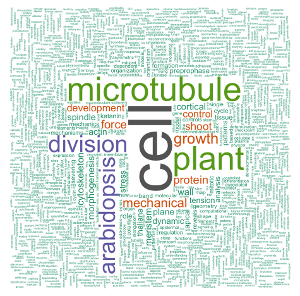
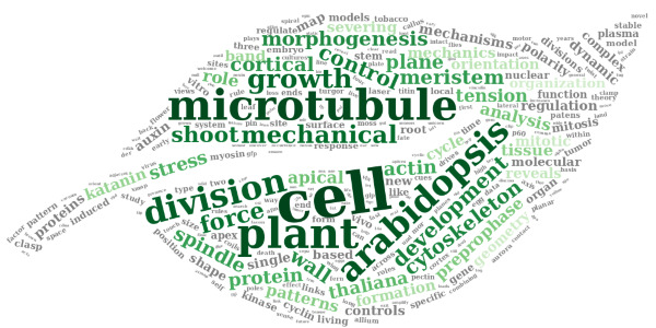
Now, let’s use {wordcloud2} with a background image. I’ll use a leaf image as background as a reference to the plant related topic of my PhD thesis. The leaf image was adapted from this other image by Sébastien Rochette, and can be downloaded here.
The snapshot of the html wordcloud is done manually on my web browser, to the targeted dimensions. I could have used {webshot}, but the use of a figure as a mask requires to refresh the browser, which is not easy with {webshot}.
figPath <- "leaf.png"l <- nrow(d)
# Change to square root to reduce difference between sizes
d_sqrt <- d %>%
mutate(freq = sqrt(freq))
my_graph <- wordcloud2(
d_sqrt,
size = 0.5, # sqrt : 0.4
minSize = 0.1, # sqrt : 0.2
rotateRatio = 0.6,
figPath = figPath,
gridSize = 5, # sqrt : 5
color = c(rev(tail(greenpal(50), 40)), rep("grey", nrow(d_sqrt) - 40)) # green and grey
# color = c(rev(tail(greenpal(50), 40)), rep(greenpal(9)[3], nrow(d_sqrt) - 40)) # green
# color = c(rev(tail(greenpal(50), 40)), rep("#FFAC40", nrow(d_sqrt) - 40)) # green and orange
)I’ve set the color to green and grey. In the commented lines, one can find two alternative choices of colors: all green, and green and orange.
Conclusion
It was great to explore this bibliography dataset three years after the end of my PhD. This was the occasion for me to learn how to play with bibliographical data with R, practice my knowledge of the tidyverse, and learn how to make wordclouds. I discovered a few things that I would not have expected, such as the fact that the median year of publication in my bibliography is only 6 years before my PhD manuscript submission and PhD defense. I also got some interesting perspectives on my work and my profile at that time.
I guess the keywords of my postdoc bibliography would also reflect plant developmental biology, but also most probably a bit more microscopy, in particular light sheet microscopy, and bioimage and data analysis. Indeed, I work even more now with image analysis tools like MorphographX and Fiji. I also work even more with the R software, with which I extend my bioimage data analysis workflows through R packages I develop like {mgx2r}, {mamut2r} or {cellviz3d}.
Acknowledgements
I would like to thank Dr. Sébastien Rochette for his help on tidying the corpus prior to generating wordclouds.
Citation:
For attribution, please cite this work as:
Louveaux M. (2018, Dec. 21). "Analysing bibliographical references with R". Retrieved from https://marionlouveaux.fr/blog/bibliography-analysis/.
@misc{Louve2018Analy,
    author = {Louveaux M},
    title = {Analysing bibliographical references with R},
    url = {https://marionlouveaux.fr/blog/bibliography-analysis/},
    year = {2018}
  }

Share this post
Twitter
Google+
Facebook
LinkedIn
Email